omXplore: a versatile series of Shiny apps to explore ‘omics’ data
Samuel Wieczorek
Thomas Burger
2025-01-31
Source:vignettes/omXplore.Rmd
omXplore.RmdAbstract
The package omXplore (standing for “Omics Explore”) is a R package which provides functions to vizualize omics data experiments. It deals with common data formats in Bioconductor such as MSnSet, MultiAssayEperiments, QFeatures or even simple lists.
Introduction
The omXplore package offers a series of built-in plots
dedicated to the visualization and the analysis of *omics (genomic,
transcriptomics, proteomics) data. As for several R packages available
in Bioconductor for exploring omics-like datasets,
omXplore is based on Shiny to make those plots easily
available in a web application. Four popular Bioconductor data objects
are currently supported: SummarizedExperiment,
MultiAssayExperiment, MSnset and
QFeatures.It is also possible to use
data.frame or matrix (or lists of) which
contains quantitative data tables (rows for features and columns for
samples).
All these formats are automatically converted into an internal S4
class which is an enriched version of the
MultiAssayexperiment class. This process is invisible to
the end-user.
The package omXplore was created to be versatile,
reusable and scalable. It differs from similar R packages in two main
points:
(versatile) The main Shiny module in
omXploreis a hub which gives access to the individual plots. The plots are automatically updated w.r.t the selected dataset (in case of data which contains several ExperimentData like the classesMultiAssayExperimentorQFeatures).(scalable) with less effort, it is easy integrate external plots (written as Shiny modules) in the main GUI of
omXplore.(reusable) Each plot (a Shiny module) can be run alone or integrated as a complementary tool in third party Shiny apps. As an example, it is well suited for the package Prostar in which it is used.
Features
omXplore provides a graphical user interface using the
Shiny and the highcharter packages for the
following visualizations:
- Connected Components of graph-type data (e.g. in proteomics datasets, graphs of peptide-protein relationship),
- Principal Component Analysis (PCA),
- Histograms to analyze the quantitative data based on cell metadata (eg missing values, imputed values, …),
- Intensity plots (boxplot and violinplot) of quantitative data. There is also a tool to select and view (by superimposition) the evolution of intensity over samples for a given set of entities,
- Density plot
- Variance distribution plot
- Heatmap
- Correlation plot
For developers or users who wants to enhance their application, additional features include:
- As each plot is a Shiny module, it can be launched in a standalone mode (from a R console) or it can be easily integrated into any third party Shiny app
- Internal convert function from a large variety of
Bioconductorobjects, - A easy way to add user-defined plots (written as Shiny modules) in
the main GUI of
omXplore
Installation
To install this package, start R (version “4.3”) and enter:
if (!require("BiocManager", quietly = TRUE))
    install.packages("BiocManager")

BiocManager::install("omXplore")
This will also install dependencies.
It is also possible to install omXplore from Github:
library(devtools)
install_github('prostarproteomics/omXplore')
Then, load the package into R environment:
Enriching native MultiAssayExperiment
The internal data struture used in omXplore is based on
the class MultiAssayExperiments
which is enriched with specific slots needed to create built-in plots.
The plots display statistical information about data contained in the
SummarizedExperiment slots of a dataset.
Some items are added to the metadata of the instance of MultiAssayExperiment and to each of the instances of SummarizedExperiment.
Additional info in MultiAssayExperiment
Currently, there is no custom slot in the metadata of the mae
contains the following additional items (in the slot names
other):
data(vdata)
MultiAssayExperiment::metadata(vdata)
## $other
## list()Additional info in SummarizedExperiment
The metadata of each SummarizedExperiment dataset contains the following items:
proteinID: the name of the column which contains xxx
colID: the name of the column which serves as unique index
cc: the list of Connected Components, based on the adjacency matrix (if exists)
type: the type of data contained in the current Experiment (e.g. peptide, protein, …)
pkg_version: the name and version number which has been used to create the current Experiment.
data(vdata)
MultiAssayExperiment::metadata(vdata[[1]])
## $pkg_version
## NULL
##
## $type
## [1] "protein"
##
## $colID
## [1] "protID"
##
## $proteinID
## [1] "protID"
##
## $cc
## $cc[[1]]
## 1 x 1 sparse Matrix of class "dgCMatrix"
## proteinID_1
## prot_1 1
##
## $cc[[2]]
## 1 x 1 sparse Matrix of class "dgCMatrix"
## proteinID_2
## prot_2 1
##
## $cc[[3]]
## 1 x 1 sparse Matrix of class "dgCMatrix"
## proteinID_3
## prot_3 1
##
## $cc[[4]]
## 1 x 1 sparse Matrix of class "dgCMatrix"
## proteinID_4
## prot_4 1
##
## $cc[[5]]
## 1 x 1 sparse Matrix of class "dgCMatrix"
## proteinID_5
## prot_5 1The adjacencyMatrix (when exists) is stored as a DataFrame in the rowData() of a SummarizedExperiment itemµ.
All modules are self-contained in the sense that it is not necessary to manipulate datasets to view the plots. The information described above are given only to discover the slots used if the user wants to enrich its dataset before using omXplore.
Using omXplore
The package omXplore offers a collection of standard
plots written as Shiny modules. The main app is a Shiny module itself
which displays the plots of each module.
This section describes how to view built-in plots and the main app of
omXplore.
Individual built-in plots
The list of plots available in the current R session via omXplore can be obtained with:
## [1] "omXplore_cc"          "omXplore_corrmatrix"  "omXplore_density"
## [4] "omXplore_heatmap"     "omXplore_intensity"   "omXplore_pca"
## [7] "omXplore_tabExplorer" "omXplore_variance"
By default, this function lists the built-in modules and the external modules compliant with omXplore.
Each of these functions is a Shiny app implemented as a module and
can be launched in a standalone mode or embedded in another shiny app
(as it is the case with the main UI of omXplore or inserted
in a third party Shiny app).
Most of these functions analyse the data contained in an Experiment
of the dataset (an instance of the class
SummarizedExperiment). For a sake of simplicity, they all
have the same two parameters: (1) the dataset in any (compatible) format
(See the help page of the plot functions for details) and (2) the indice
of the assay to analyse (See MultiAssayExperiment).
Internally, each function builds the enriched instance of MAE used inside omXplore then show the plot for the assay which has been specified in parameters.
data(sub_R25)
app <- omXplore_density(sub_R25, 1)
shiny::runApp(app)
Note: this code to run a shiny app follows the recommendations of Bioconductor on Running Shiny apps.
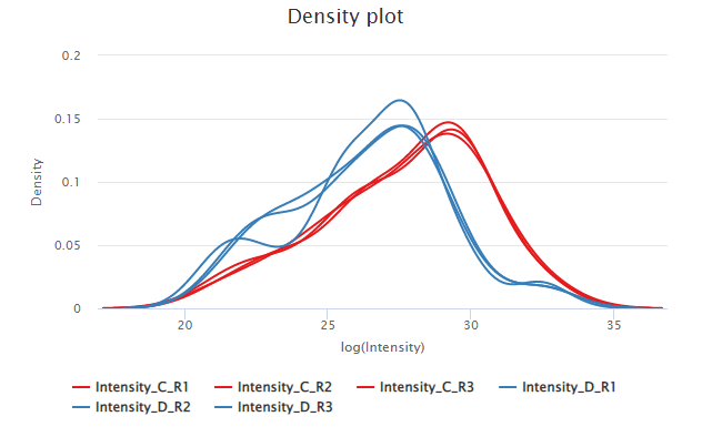
Plot generated by the module omXplore_density()
Main UI
As it is 9described in the previous section, omXplore have several built-in plots. And it may be fastidious to launch each plot function one after one to completely analyze a dataset.
For that purpose, omXplore has another shiny app, called
view_dataset() which acts as a hub for plots to facilitate
the analyse of the different assays in a dataset. It is launched as
follows:
data(sub_R25)
app <- view_dataset(sub_R25)
shiny::runApp(app)
The resulting UI is the following:
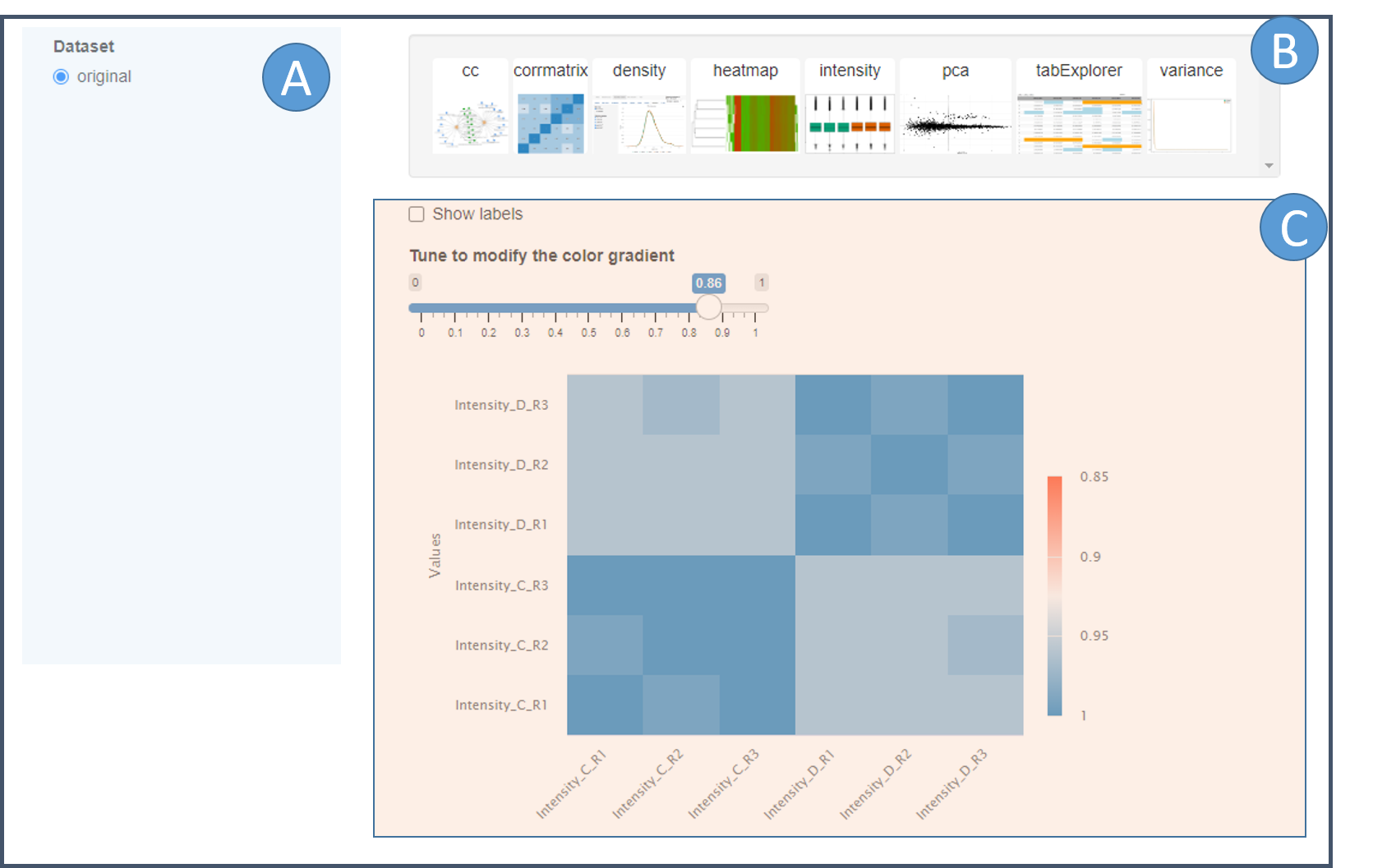
omXplore interactive interface with modal.
The interface is divided in three parts.
(A) Choosing the assay
A widget let the user select one of the experiments contained in the dataset.
(B) Select which plot to display
A series of clickable vignettes which represent the different plots available. When the user clicks on a vignette, the corresponding plot is displayed (See are C).
(C) Viewing the plots
The plots are displayed in the same window as the UI (below the
vignettes) or in a modal window, depending of the option used to launch
the Shinyp app (See ?view_dataset).
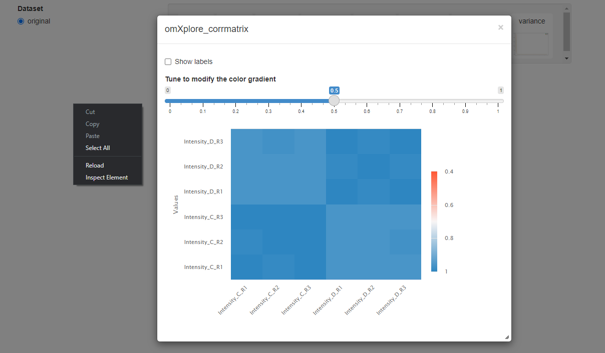
omXplore interactive interface with modal.
When a plot is displayed, it shows the data corresponding to the dataset selected in the widget (of the left side). If this dataset is changed, the plot is automatically updated with the data of the new dataset.
Session information
## R version 4.4.2 (2024-10-31)
## Platform: x86_64-pc-linux-gnu
## Running under: Ubuntu 24.04.1 LTS
##
## Matrix products: default
## BLAS:   /usr/lib/x86_64-linux-gnu/openblas-pthread/libblas.so.3
## LAPACK: /usr/lib/x86_64-linux-gnu/openblas-pthread/libopenblasp-r0.3.26.so;  LAPACK version 3.12.0
##
## locale:
##  [1] LC_CTYPE=C.UTF-8       LC_NUMERIC=C           LC_TIME=C.UTF-8
##  [4] LC_COLLATE=C.UTF-8     LC_MONETARY=C.UTF-8    LC_MESSAGES=C.UTF-8
##  [7] LC_PAPER=C.UTF-8       LC_NAME=C              LC_ADDRESS=C
## [10] LC_TELEPHONE=C         LC_MEASUREMENT=C.UTF-8 LC_IDENTIFICATION=C
##
## time zone: UTC
## tzcode source: system (glibc)
##
## attached base packages:
## [1] stats     graphics  grDevices utils     datasets  methods   base
##
## other attached packages:
## [1] omXplore_0.99.93 BiocStyle_2.34.0
##
## loaded via a namespace (and not attached):
##   [1] RColorBrewer_1.1-3          jsonlite_1.8.9
##   [3] MultiAssayExperiment_1.32.0 magrittr_2.0.3
##   [5] shinyjqui_0.4.1             estimability_1.5.1
##   [7] MALDIquant_1.22.3           rmarkdown_2.29
##   [9] fs_1.6.5                    zlibbioc_1.52.0
##  [11] ragg_1.3.3                  vctrs_0.6.5
##  [13] htmltools_0.5.8.1           S4Arrays_1.6.0
##  [15] curl_6.2.0                  broom_1.0.7
##  [17] SparseArray_1.6.1           mzID_1.44.0
##  [19] TTR_0.24.4                  sass_0.4.9
##  [21] KernSmooth_2.23-24          bslib_0.9.0
##  [23] htmlwidgets_1.6.4           desc_1.4.3
##  [25] plyr_1.8.9                  impute_1.80.0
##  [27] emmeans_1.10.6              zoo_1.8-12
##  [29] lubridate_1.9.4             cachem_1.1.0
##  [31] igraph_2.1.4                mime_0.12
##  [33] iterators_1.0.14            lifecycle_1.0.4
##  [35] pkgconfig_2.0.3             Matrix_1.7-1
##  [37] R6_2.5.1                    fastmap_1.2.0
##  [39] shiny_1.10.0                GenomeInfoDbData_1.2.13
##  [41] MatrixGenerics_1.18.1       clue_0.3-66
##  [43] digest_0.6.37               pcaMethods_1.98.0
##  [45] colorspace_2.1-1            S4Vectors_0.44.0
##  [47] textshaping_1.0.0           GenomicRanges_1.58.0
##  [49] timechange_0.3.0            httr_1.4.7
##  [51] abind_1.4-8                 compiler_4.4.2
##  [53] doParallel_1.0.17           backports_1.5.0
##  [55] BiocParallel_1.40.0         viridis_0.6.5
##  [57] dendextend_1.19.0           gplots_3.2.0
##  [59] MASS_7.3-61                 DelayedArray_0.32.0
##  [61] scatterplot3d_0.3-44        gtools_3.9.5
##  [63] caTools_1.18.3              mzR_2.40.0
##  [65] flashClust_1.01-2           tools_4.4.2
##  [67] PSMatch_1.10.0              httpuv_1.6.15
##  [69] quantmod_0.4.26             FactoMineR_2.11
##  [71] glue_1.8.0                  promises_1.3.2
##  [73] QFeatures_1.16.0            grid_4.4.2
##  [75] cluster_2.1.6               reshape2_1.4.4
##  [77] generics_0.1.3              gtable_0.3.6
##  [79] preprocessCore_1.68.0       shinyBS_0.61.1
##  [81] sm_2.2-6.0                  tidyr_1.3.1
##  [83] data.table_1.16.4           XVector_0.46.0
##  [85] BiocGenerics_0.52.0         foreach_1.5.2
##  [87] ggrepel_0.9.6               pillar_1.10.1
##  [89] stringr_1.5.1               limma_3.62.2
##  [91] later_1.4.1                 dplyr_1.1.4
##  [93] lattice_0.22-6              tidyselect_1.2.1
##  [95] vioplot_0.5.0               knitr_1.49
##  [97] gridExtra_2.3               bookdown_0.42
##  [99] IRanges_2.40.1              ProtGenerics_1.38.0
## [101] SummarizedExperiment_1.36.0 stats4_4.4.2
## [103] xfun_0.50                   Biobase_2.66.0
## [105] statmod_1.5.0               factoextra_1.0.7
## [107] MSnbase_2.32.0              matrixStats_1.5.0
## [109] DT_0.33                     visNetwork_2.1.2
## [111] stringi_1.8.4               UCSC.utils_1.2.0
## [113] lazyeval_0.2.2              yaml_2.3.10
## [115] evaluate_1.0.3              codetools_0.2-20
## [117] MsCoreUtils_1.18.0          tibble_3.2.1
## [119] BiocManager_1.30.25         affyio_1.76.0
## [121] multcompView_0.1-10         cli_3.6.3
## [123] xtable_1.8-4                systemfonts_1.2.1
## [125] munsell_0.5.1               jquerylib_0.1.4
## [127] Rcpp_1.0.14                 GenomeInfoDb_1.42.3
## [129] XML_3.99-0.18               parallel_4.4.2
## [131] leaps_3.2                   pkgdown_2.1.1
## [133] ggplot2_3.5.1               assertthat_0.2.1
## [135] AnnotationFilter_1.30.0     bitops_1.0-9
## [137] viridisLite_0.4.2           mvtnorm_1.3-3
## [139] rlist_0.4.6.2               affy_1.84.0
## [141] scales_1.3.0                xts_0.14.1
## [143] ncdf4_1.23                  purrr_1.0.2
## [145] highcharter_0.9.4           crayon_1.5.3
## [147] rlang_1.1.5                 vsn_3.74.0
## [149] shinyjs_2.1.0